Breast Cancer Detection — CNN transfer learning on CBIS-DDSM

01 / the honest version

What this is,
and what it isn't

This is university coursework. A convolutional neural network trained on a public mammography dataset, built to learn the deep-learning workflow end to end. It is not a diagnostic tool, it has never been near a patient, and it is not close to state of the art.

It set out to match a published benchmark — AUC 0.844 from Falconí et al. on the same dataset — and reached 0.77. That gap is the most interesting thing on this page, so it is stated up front rather than buried.

The project was marked 74%. Worth noting only because of what it says about how this kind of work is judged: the mark reflects method, iteration and reporting, not whether the number came out where I wanted it.

Why show a project that missed its target

Because the method was sound and the reporting is honest, and those are the things that transfer. The pipeline was built in deliberate stages with each change measured against the last, one promising technique made results worse and was kept in the record, and the model's attention was inspected rather than trusted. A tidier number would say less.

02 / the data

CBIS-DDSM

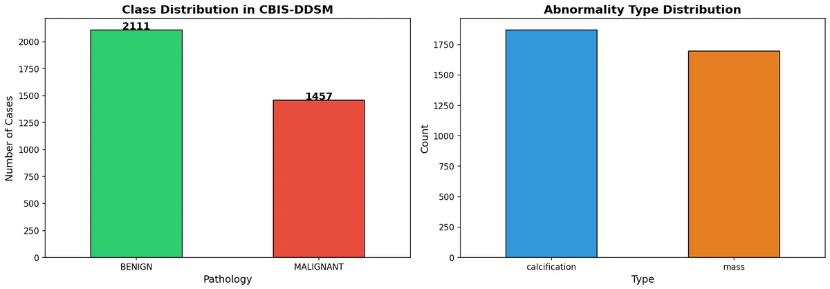
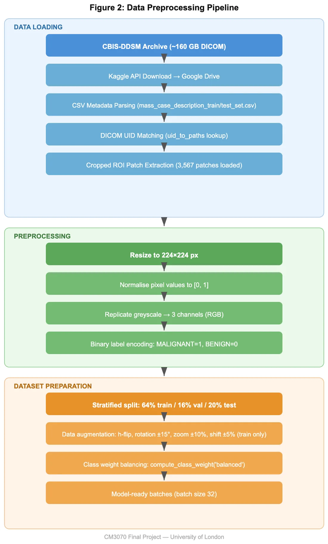
The Curated Breast Imaging Subset of DDSM — a public, de-identified set of screening mammograms with pathology-confirmed labels. 3,567 images were loaded and split 2,282 train / 571 validation / 714 test, stratified so class balance holds across all three.

The classes are uneven — roughly 59% benign to 41% malignant — so training used class weights, and accuracy was rejected as a headline metric from the start. A model that called every scan benign would score 59% accuracy while catching no cancer at all.

Bar chart of benign versus malignant image counts in the CBIS-DDSM subset — Class distribution across the loaded dataset.

Diagram of the data preparation pipeline from raw DICOM through resizing and augmentation — Preparation: decode, resize to 224×224 for VGG16, normalise, augment. open full size ↗

03 / method

Four stages,
each measured

Rather than reaching for the largest available model, the pipeline was built in rungs — each one a single change from the rung below, so any movement in the score could be attributed to something specific.

STAGE 01

Baseline CNN

A small convolutional network trained from scratch. Establishes the floor and proves the data pipeline works before any transfer learning is involved.

STAGE 02

VGG16, frozen

ImageNet weights held fixed, a new classifier head trained on top. Tests whether generic visual features transfer to mammography at all.

STAGE 03

+ regularisation

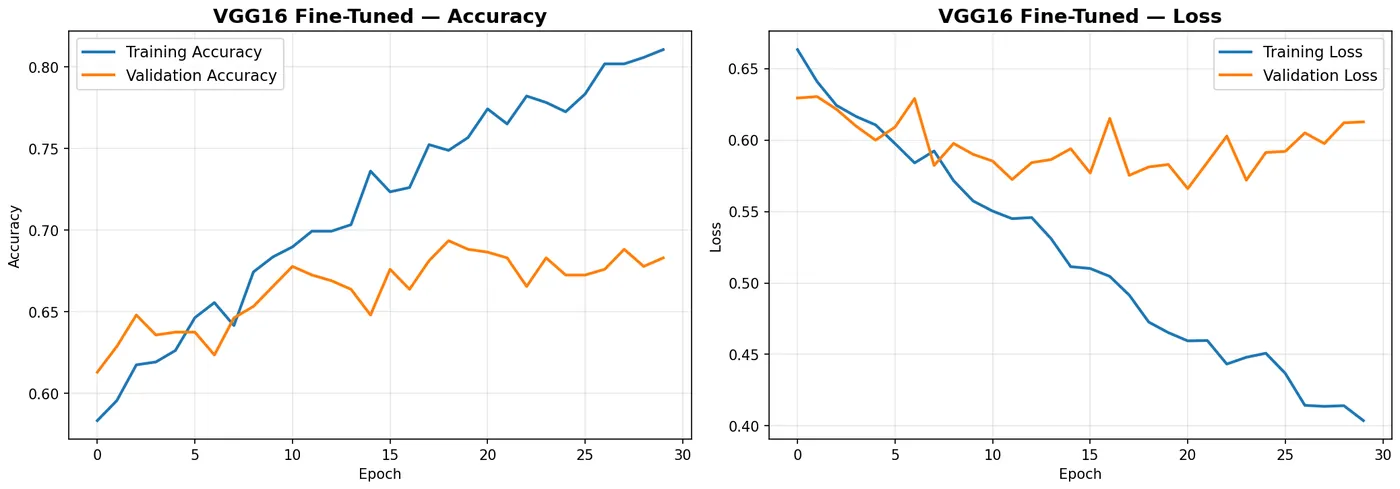
Dropout and L2 added after the frozen model overfit — training accuracy climbing while validation stalled.

STAGE 04 · BEST

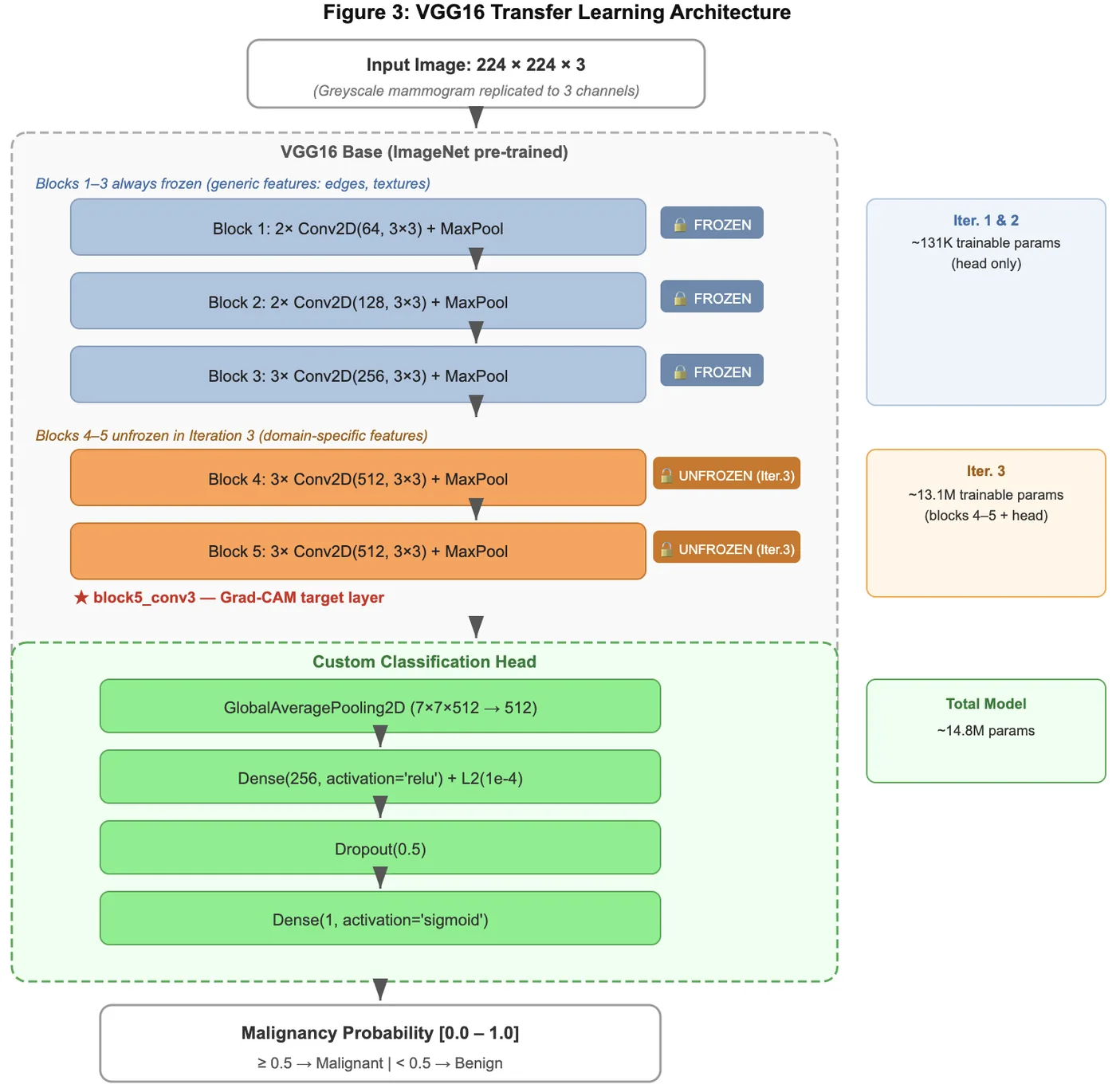
VGG16, fine-tuned

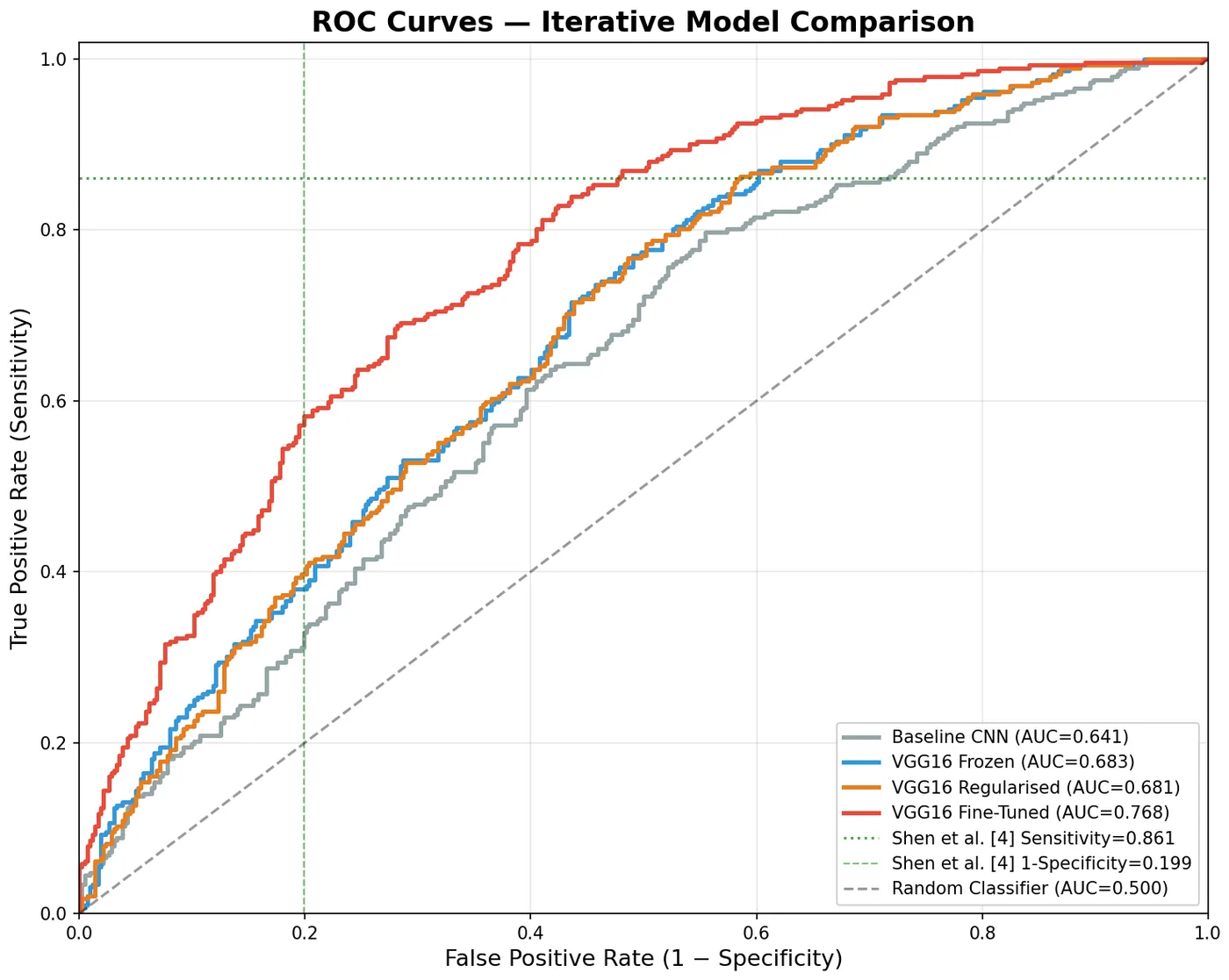
AUC 0.768

Blocks 4 and 5 unfrozen at a low learning rate, so the later, more task-specific filters adapt to tissue.

Three further techniques were tried on top: an ensemble of the strongest models (AUC 0.774, the best overall result), test-time augmentation, and CLAHE contrast enhancement. Only the ensemble helped meaningfully.

Diagram of the VGG16 architecture with the fine-tuned blocks highlighted — VGG16, with the blocks unfrozen during fine-tuning. open full size ↗

Training and validation curves for the fine-tuned VGG16 model — Training and validation curves for the fine-tuned model.

04 / results

0.77, and what
that means

AUC in one sentence

Take one real cancer scan and one real benign scan at random: AUC is the probability the model gives the cancer the higher malignant score. At 0.77 it gets that ordering right roughly 77 times in 100. A coin flip is 0.50. It is the headline metric here precisely because it needs no threshold — unlike accuracy, it cannot be flattered by the majority class.

Model	AUC	Note
Baseline CNN	—	Floor: proves the pipeline, not the science
VGG16 frozen	—	Generic features transfer, but overfit quickly
VGG16 + regularisation	—	Overfitting controlled
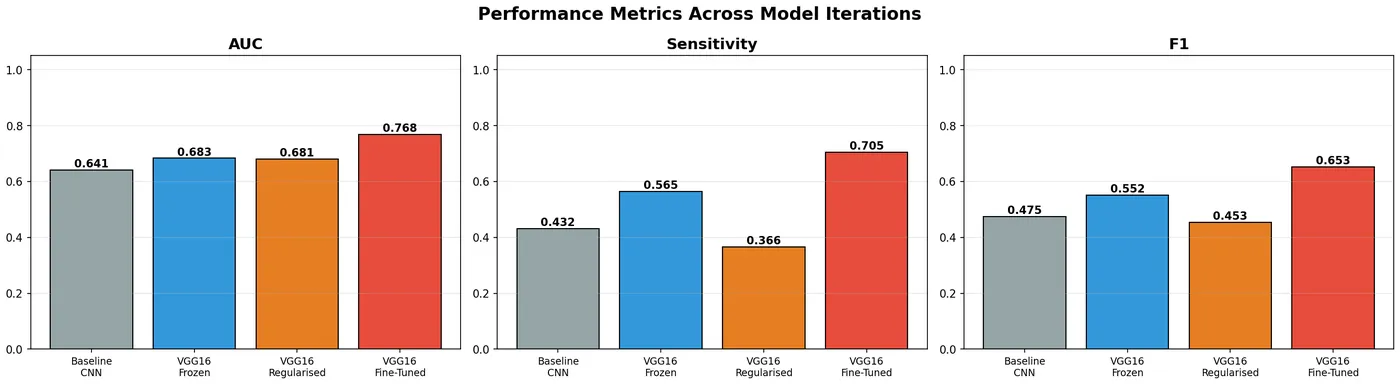
VGG16 fine-tuned	0.768	Best single model · sensitivity 0.71
Ensemble	0.774	Best overall
Literature target (Falconí et al.)	0.844	Not reached

ROC curves comparing the models against each other — ROC across the pipeline. The curve is the sensitivity / false-alarm tradeoff swept across every threshold; AUC is the area beneath it.

Bar chart comparing accuracy, precision, recall and F1 across experiments — Metric comparison across experiments.

Why sensitivity matters more than accuracy here

Sensitivity is the share of real cancers the model catches. At 0.71, roughly 85 of the 292 malignant scans in the test set were called benign. In screening, that error costs far more than a false alarm: a false positive leads to another look, a false negative leads to nothing at all. Any honest reading of this project leads with that number, not with accuracy.

05 / the negative result

CLAHE made it
worse

Contrast Limited Adaptive Histogram Equalisation is a standard preprocessing step in medical imaging — it boosts local contrast and, in principle, should make lesion boundaries easier for a network to find. It is widely used and it was a reasonable thing to try.

It reduced performance here. Both the CLAHE-only and CLAHE-plus-augmentation runs scored below the equivalent runs without it.

Kept, not quietly dropped

The experiment stays in the record because a technique that should have worked and didn't is a real finding about this data. The plausible reading is that aggressive local contrast enhancement amplified noise and acquisition artifacts alongside tissue detail — but that was not tested, so it is offered as a hypothesis and not a conclusion.

06 / explainability

Where the
model looked

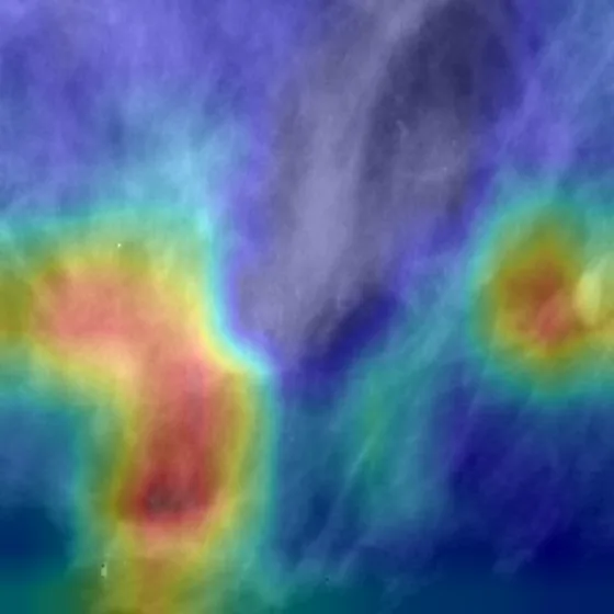
Grad-CAM answers one question: which parts of the image drove the prediction? Red is where the model looked hardest. It is the difference between a model that learned something anatomical and one that found a shortcut — and it is the only reason the flaw in the limitations section below was ever noticed.

Pick a case. Confidence is shown throughout as P(malignant); the decision threshold is 50%.

TRUTH

—

MODEL SAID

—

P(MALIGNANT)

—

0% · certainly benign50% · thresholdcertainly malignant · 100%

The most instructive case is the one it got wrong

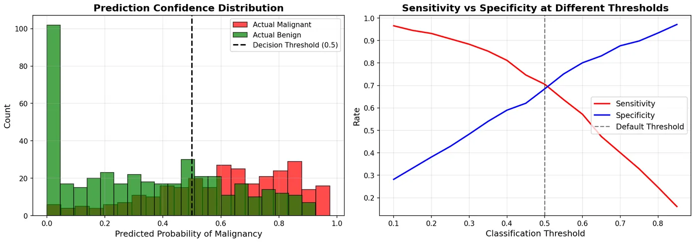
fp-52 is a benign scan the model called malignant — at 52.4% against a 50% threshold. It was 2.4 points from undecided, and the threshold made the call on its behalf. In a confusion matrix that case counts exactly the same as a confident blunder, because turning a probability into a label throws the probability away. That is the clearest argument on this page for reporting AUC rather than accuracy.

Failure analysis chart showing the distribution of model errors — Failure analysis across the held-out set.

07 / limitations & ethics

What this
cannot do

This model must not be used to make any decision about a person. It is coursework trained on a public research dataset, evaluated once on a held-out split, and never validated on an external population, a different scanner, or a different clinic. Performance is well below clinical grade.

CBIS-DDSM carries the biases of its origin — a curated research collection drawn from a specific population and imaging era. A model trained on it should not be assumed to behave the same way on scans from anywhere else. No demographic breakdown of performance was performed, so any claim about fairness across groups would be unsupported.

A defect found after submission

While preparing these figures, two of the sample images turned out not to be mammograms at all, but ROI masks — the outline a radiologist drew around a lesion. The cause is in the data loader: it resolves each record to a folder and takes the first file in it, and in this dataset that folder holds both the cropped scan and its mask. In a sample of ten images, two were masks.

The exact contamination rate across the full set has not yet been measured, and the fix and re-run are scheduled. It is reported here because it is a plausible contributor to the gap between this project's 0.77 and the 0.844 it aimed at — and because every metric looked healthy while it was happening. Only the attention maps gave it away.

What I would do next

Fix the loader so the file is resolved by name rather than position, measure the true contamination rate, and re-run the identical protocol so the comparison against 0.768 is fair. Then add a sample-grid assertion at the front of the pipeline so this class of bug cannot recur silently. If the number moves, the gap is explained; if it does not, a confound has been eliminated and the honest conclusion stands more firmly.

What this is,and what it isn't